

Averaging values in an Excel sheet is easy. But perhaps you want to ignore zeros or include multiple sheets. Knowing how each averaging function works is the key to choosing the right one.

Image: iStock/Aajan
Averaging isn’t always a simple total divided by the number of items totaled. Fortunately, Microsoft Excel offers several averaging functions, and one of them will probably get the job done. In this article, we’re going to briefly review the basic AVERAGE() function, which you’re probably already familiar with. Then, we’ll look at AVERAGEA(), AVERAGEIF() and AVERAGEIFS().
SEE: 69 Excel tips every user should master (TechRepublic)
I’m using Microsoft 365 on a Windows 10 64-bit system, but you can use earlier versions. You can download the demonstration .xlsx and .xls file, or work with your own data. All of these functions are supported by the browser.
How to use AVERAGE() in Excel
The best place to start is with the most basic function, AVERAGE(); this function averages a set of values by adding those values and then dividing by the number of values. You learned this expression in grade school, and you’re probably familiar with this function already.
The AVERAGE() function evaluates values by range or individual references:
AVERAGE(range)
AVERAGE(value1,[ value2]…, )
Text, logical values, and empty cells are ignored. If there’s an error value in the referenced list AVERAGE() returns an error.
Using the simple set of values in Figure A, the AVERAGE() function in D3
=AVERAGE(B3:B9)
returns the average 4.8. The average function evaluates the zero but ignores the blank cell and the logical value TRUE. In this case, AVERAGE() returns the sum of the five values—1, 6, 0, 7, and 10—divided by 5: 24/5.
What happens if you want the TRUE value evaluated? Let’s look at a function solution for that situation next.
Figure A
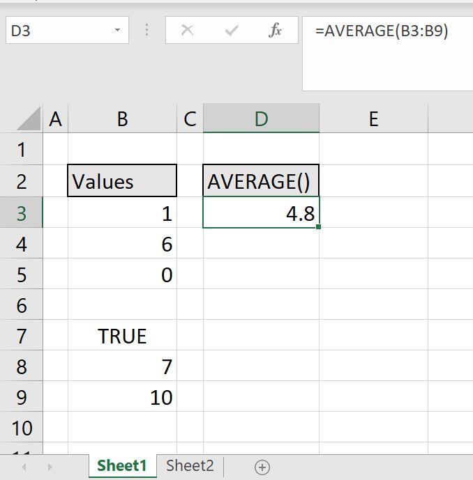
A simple average ignores blanks and evaluates 0.
How to use AVERAGEA() in Excel
Excel’s AVERAGEA() purpose and syntax are similar to AVERAGE(). The main difference is that AVERAGEA() evaluates the logical values TRUE and FALSE as 1 and 0, respectively. Figure B shows the result of the AVERAGEA() function on the same data set. However, this time, the TRUE logical value equals 1 and is evaluated. Consequently, the same data set evaluates to 25/6.
SEE: How to average unique values in Excel the easy way (TechRepublic)
Figure B
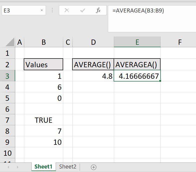
AVERAGEA() evaluates the TRUE value.
How to use AVERAGEIF() in Excel
Both of the previous average functions evaluate zero. The value zero adds nothing to the sum but adds 1 to the divisor. There’s no averaging function that ignores 0, but it’s easy to do so using AVERAGEIF(). This function returns the average of a data set when those values meet a specific condition. This function uses the syntax
AVERAGEIF(range, criteria, [average_range])
where range references the values to be averaged, criteria specifies the condition, and [average_range] is an optional range of values to be averaged. Figure C shows the function
=AVERAGEIF(B3:B9,”<>0″)
used to average the same data set without evaluating 0. In this case, this function evaluates to 24/4 because the zero value isn’t evaluated.
Figure C
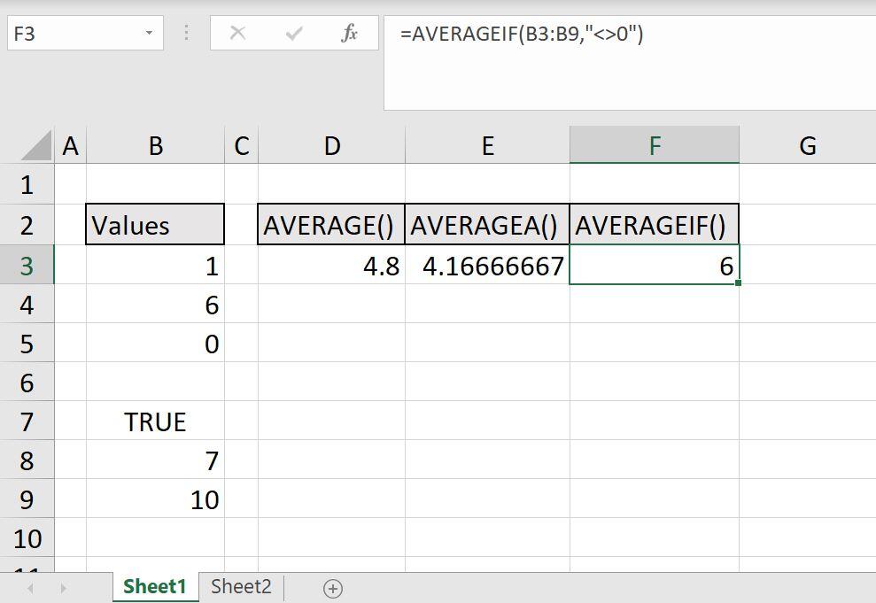
Use AVERAGEIF() to narrow the set of data values.
AVERAGEIF() was introduced in 2007, so it’s not available in the menu version.
How to use AVERAGEIFS() in Excel
The AVERAGEIFS() function is similar to AVERAGEIF() in purpose but allows multiple criteria:
AVERAGEIFS(average_range, criteria_range1, criteria1, [criteria_range2, criteria2], …)
The first three arguments specify the range of values to be averaged, the criteria range to be evaluated, and the criteria. The optional arguments allow you to specify additional criteria ranges and criteria. Our simple data set doesn’t include three ranges, which might seem a bit confusing. In this case, average_range and criteria_range1 will be the same, as you can see in Figure D.
Figure D
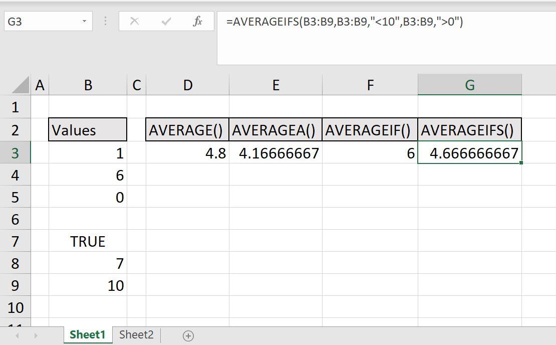
AVERAGEIFS() lets you specify multiple conditions.
The function in G3, =AVERAGEIFS(B3:B9,B3:B9,”<10″,B3:B9,”>0″), averages the same data set, but evaluates only those values that are less than 10 and greater than zero. In other words, this function evaluates only 1 through 9. Consequently, the function evaluates to 14/3.
Values are included in the sum and the divisor only if they meet the criteria conditions. In both cases, the criteria argument is a literal string. You could just as easily reference an input cell to make things more dynamic.
How to do 3D averaging in Excel
When you’re working with multiple sheets, there’s good news and there’s bad news. First, the good news, AVERAGE() and AVERAGEA() support multiple sheets:
D4: =AVERAGE(Sheet1:Sheet2!B3:B9)
E4: =AVERAGEA(Sheet1:Sheet2!B3:B9)
as shown in Figure E. (When entering the function, hold down the Shift key, and click the sheet tabs to access data sets beyond the active sheet.) The bad news that the two conditional functions in F4 and G4 don’t support 3D averaging.
Figure E
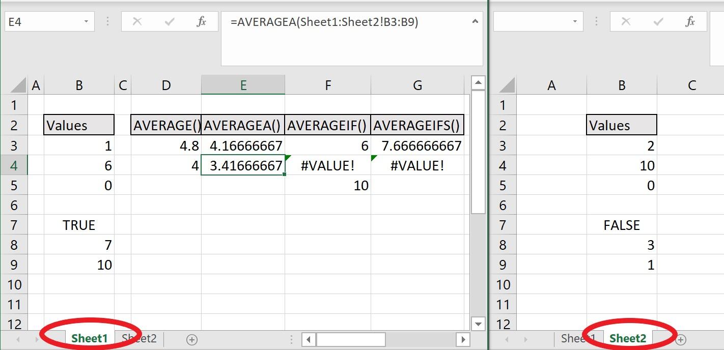
AVERAGE() and AVERAGEA() support 3D references.
Averaging is simple. Knowing what each function does and how it evaluates special values such as 0, a blank cell, and TRUE/FALSE is the key to using the right function. Unfortunately, neither of the conditional functions, support 3D referencing. In a future article, we’ll address this problem.
Also see
This article is auto-generated by Algorithm Source: www.techrepublic.com